
统计降水降尺度 三种 Perfect Prognosis 方法的评估
编辑这篇文章主打的核心就是 可迁移性(transferability),通俗解释是,我们训练SD方法时使用的是过去的气候数据,如果未来气候的变化超出了历史数据的范围,这些方法还能正确地预测未来的降水吗?但这个解释太笼统了,我们从头来解释一下
可迁移性(transferability)
我们用过去几十年的气候数据(如1979-2008年的气温、湿度、风速等)来训练统计模型,让它学会大尺度气候模式如何影响局地降水。如果这个模型能正确地应用到未来的气候预测中(如2071-2100年),说明它是可迁移的。但如果它预测未来时出现了偏差,那就说明它的可迁移性一般。
可迁移性问题的核心在于:未来的气候条件可能会超出模型在历史数据中学到的规律,导致模型无法正确适应新变化。这个问题可以从三个方面来理解。
(1) 气候情况本身的根本性变化。比如说,我们只学习了加减乘除,但是考试第一题考微积分,这不完蛋了。同理,如果未来气候超出了它的经验范畴,那就预测不准。比如说厄尔尼诺在过去只出现过几十次,但是由于全球气候变暖,现在每年都来一下,我们用过去30年训练好的模型来做现在的预测,那就测不准。
(2) GCM偏差的动态性。除了气候情况的变化外,GCM偏差也是同理,GCM在未来的偏差可能与过去不同,所以模型在实际预测时不知道如何修正这些新偏差(没学过),即训练时的GCM误差不等于未来的GCM误差,模型可能无法正确补偿误差。
(3) 统计关系的改变。由于气候变化,predictor和predictand之间的关系也不一样了,统计模型在训练时"记住"的关系不等于未来预测时真实的关系,也就是统计模型本身可能不适应未来的变化。
所以针对统计模型在可迁移性方面的研究还是很重要的,毕竟像训练得再好、实际却不能用这样的模型搞出来没意义。因此这个论文针对广义线性模型(GLMs)、卷积神经网络(CNNs)、后验随机森林(APRFs)可迁移性进行了讨论。
最后结果表明:APRFs表现最好,在历史数据上(交叉验证)CNNs和APRFs的表现比GLMs更好,说明考虑非线性关系对降尺度很重要。GCM数据上(非完美条件)APRFs能够较好地纠正GCM的偏差,使预测结果更接近实际观测数据。APRFs预测的未来降水变化趋势最稳定,三种方法的预测结果都和GCM的原始模拟结果大致一致,说明它们能够正确地反映未来的气候变化趋势,但GLMs和CNNs在某些地点会放大气候变化信号,而APRFs的预测更稳定、更符合GCM原始数据。不过APRFs需要改进时间一致性——现有的APRFs在模拟降水的连续性(干湿天转换)时表现不好。他们提出了一个简单改进方法,称为TAPRFs,它可以更准确地模拟干湿天转换概率,使降水序列更符合实际气象观测。
这是概览,下面是精读。
精读
These relationships are learned over a historical period, and thus a relevant question is whether they can be transferred to the future GCM simulations, that is, whether climate changes produced by GCMs (e.g., changes in mean rainfall) are broadly preserved by the downscaling methods.
这些关系在历史周期内被学到,因此相关问题是,他们是否可以被传递到 GCM 的未来模拟中? 也就是说,降尺度方法是否能够广泛的保留GCM输出的气候变化?比如 降雨量的变化。
这句话其实还是 transferability 的内容,相当于在问,对于降尺度方法模型,我们是用历史数据训练得到的,没有问题,但是现在应用到 GCM 输出数据时候,是否仍然能够保持 GCM 预测的气候变化趋势?或者说,它会不会修改 GCM 给出的结果?
举个例子,虽然GCM 分辨率低,但是他还是能预测出来巴黎年均降水量会减少 10%,我们现在用降尺度来提高分辨率,结果数据变成了年均降水量增加 5%,这和 GCM的结果不匹配了,降尺度的任务就是老老实实提高分辨率,GCMs 的结果是通过动力物理方程来的,应该是很准的,让你降尺度模型这么一搞反而大错特错了。
现在就有一个问题,为什么降尺度方法可能会改变GCM预测的气候变化?这就是我们上面已经分析过的可导致可迁移性问题的三个方面。如果更详细地说,降尺度一个重要功能是纠正偏差,但是如果方法选得不好,可能把GCM预测的气候变化信号也一起改掉了。
Wootten et al. (2020) and Hernanz et al. (2022) performed a comprehensive evaluation of different machine learning alternatives, the latter concluding that the choice of technique can affect the downscaled results up to the point of producing climate change signals of reverse sign for precipitation. Moreover, even for the same SD technique, Manzanas, Fiwa, et al. (2020) showed that the choice of predictor variables considered can also lead to dramatically different precipitation projections.
ML方法的选择和同一SD下predictor的选择都会影响降尺度结果,选错了方法,甚至会产生相反符号的降水气候变化信号。
In this context, Legasa et al. (2022) recently introduced a posteriori random forests (APRFs). APRFs are a modification of the random forest (RF) machine learning technique (Breiman, 2001) similar to quantile random forests (Meinshausen, 2006) able to model the whole parametric probability distribution of the target variable.
也就是说,这个论文的工作是建立在 Legasa et al. (2022) 他以前的工作基础上的,其论文链接: A Posteriori Random Forests for Stochastic Downscaling of Precipitation by Predicting Probability Distributions
这里补充知识: 随机森林算法
On top of their interpretability and their skill capturing non-linear predictor-predictand relationships, RFs automatically perform feature/predictor selection, thus avoiding the complex, time-consuming and often human-guided task of pre-defining an informative set of predictors.
后验随机森林有几个显著的好处。首先是容易理解,叫做interpretability,比如说决策过程、推理过程、结果合理性。这里主要体现的是,随机森林可以计算出哪些变量(predictors)最重要,比如降水预测中,温度、湿度、风速等哪个因素影响最大,因此它可以自动选择predictor。PS:神经网络可解释性差,属于黑箱子。其次是能捕捉非线性关系。
Nevertheless, Legasa et al. (2022) tested APRFs using reanalysis predictors, thoroughly assessing the calibration/training stage, and thus a relevant next question is whether this technique is also suitable for SD of climate change scenarios, that is, using GCM predictors.
随机森林的评估工作已经被原作者做完了,所以这里他们做 transferability 方面的评估
The present article assesses this topic for precipitation, a variable notably difficult to model (see, e.g., Gutiérrez et al., 2019; Legasa et al., 2022) due to its semi-continuous nature (a continuous probability distribution for wet days with positive mass at 0 accounting for dry days) and the limited predictive capability of the large-scale predictors (see Gutiérrez et al., 2019; Themeßl et al., 2011; Vaittinada Ayar et al., 2016 and the references in the next paragraphs).
降水这个变量非常难建模,主要有两个核心原因。降水是半连续的(semi-continuous nature):湿天(wet days)的降水量符合一个连续概率分布,而干天(dry days)的降水量为0(在0处有一个正质量点positive mass at 0)。即,当这一天从没有降水(0mm)变到有降水(5mm)这个过程,是不连续的。后面就会看到,他们用两个模型来分别做分类(下不下雨)和连续分布(降雨量)。
大尺度气候变量对降水的预测能力有限(limited predictive capability of the large-scale predictors):降水是一个高度局部化的现象,GCM无法精准预测局地降水。补充:大尺度变量predictor和局地降水的关系不一定稳定。比如以前升2°就下雨,现在升1°就下,这个统计关系不再符合了。
Pham et al. (2019) compared linear discriminant analysis, SVMs and RFs, concluding that RFs outperformed the other methods when used to downscale rainfall discretized in 3 states (dry, non extreme rainfall, extreme rainfall).
Xu et al. (2020), instead, assessed three methods (RFs, SVMs, and a deep learning architecture) for downscaling future precipitation under two RCPs, concluding that SVMs were the preferred option. Nevertheless, these two studies used traditional RFs instead of APRFs, which allow us to model the whole distribution of precipitation.
Xu et al. (2020)他们用的 RFs,没用APRFs,说不定 APRFs 能更好,这就是说我们做 APRFs 的意义
The present article aims to fill this gap of knowledge by assessing the suitability of APRFs to produce local climate change scenarios of precipitation over Europe, using 83 meteorological stations and the RCP8.5 scenario from EC-Earth. Moreover, APRFs are put in context with two other relevant machine learning methodologies: the well-established general linear models (GLMs, Chandler, 2005) and the widely used convolutional neural networks (CNNs, Lecun et al., 1998).
这就有问题了,83个欧洲各地的气象站,每个气象站的数据是独立使用的。每个气象站都会有一组对应的历史降水观测数据(真实记录),以及来自GCM(EC-Earth)的大尺度气候预测变量(如温度、湿度、风速等)。这样为每个气象站分别训练一个降尺度模型,然后再评估降尺度方法(GLMs, CNNs, APRFs)哪个更好。
RCP8.5(Representative Concentration Pathway,代表性浓度路径)是IPCC(政府间气候变化专门委员会)提出的未来温室气体排放情景。表示到2100年,地球的辐射强迫(气候变暖的主要驱动因素)增加8.5 W/m²,对应的是最极端的高排放情况。
EC-Earth作为一个全球气候模式,可以运行不同的RCP情景,比如RCP2.6(低排放)、RCP4.5(中等排放)、RCP8.5(高排放)。本文采用的是EC-Earth在RCP8.5情景下的模拟数据,用于研究在高排放情况下,未来欧洲的降水变化趋势。
后面2.1数据集选择部分略过,没啥意思。
This selection includes circulation variables, which are less affected by orography and model resolution, together with thermodynamic ones, which are linked to changes in the radiation budget and need to be considered in climate change studies (Huth, 2004).
选预测因子为环流变量的好处是它们受地形和模式分辨率影响较小。
偏差校正方法
X_{GCM}:EC-Earth GCM预测的变量(如温度、风速等)。
\text{mean}(X_{\text{HISTORICAL}}^{\text{month}}):GCM在历史时期(1979-2008年)该月份的平均值。
\text{mean}(X_{\text{REANALYSIS}}^{\text{month}}):ERA-Interim再分析数据在该月份的平均值。
\hat{X}_{GCM}:校正后的GCM预测变量。
这个公式的本质是对EC-Earth GCM的预测变量进行偏差校正,使其更符合ERA-Interim(再分析数据)在历史时期的统计特征,以减少GCM在年度循环(年周期)上的误差。
更精细地来说,我们把ERA-Interim再分析数据当作观测真实数据,来对GCM的预测变量进行校正。
这个公式其实基于一个简单的偏差修正(bias correction)方法,核心思想是:首先计算GCM的历史偏差(基于ERA-Interim):
GCM在历史时期的系统性偏差 = GCM在历史时期(1979-2008年)该月份的平均值 - ERA-Interim再分析数据在该月份的平均值。然后用这个偏差修正GCM的数据: \hat{X}_{GCM} = X_{GCM} - \text{bias}
Note that this simple transformation, applied to both the historical and RCP8.5 predictors, brings the first-order moment of the reanalysis and the GCM into agreement, thereby providing a better approximation for the perfect prognosisassumption of relying on predictors well represented by the GCM (Gutiérrez et al., 2019; Manzanas, Fiwa, et al., 2020).
这次简单的修正变换使得GCM和ERA-Interim在一阶矩(first-order moment)(期望/均值)上保持一致,让GCM变量的统计特征更接近真实气候,减少系统性偏差。GCM的系统性偏差小了,那么PP假设的核心——统计降尺度方法假设GCM的大尺度变量(如风速、湿度)可以很好地表示真实气候——就更加成立(如果GCM变量偏差太大,这个假设就不成立,降尺度预测也会不准)。
EC-Earth was re-gridded from its native spatial resolution (1.12°) to the ERA-Interim's grid considered in VALUE (2°) using bilinear interpolation.
EC-Earth GCM的原始分辨率是1.12°,但ERA-Interim再分析数据的分辨率是2°。为了匹配ERA-Interim的数据,用"双线性插值"(bilinear interpolation)把EC-Earth数据重新网格化(re-grid)到2°分辨率,让GCM和ERA-Interim数据在空间上对齐。
降水的概率分布建模
降水数据的概率分布建模,使用伯努利-伽马分布(Bernoulli-Gamma distribution)来描述降水特性。这个我们之前已经提到过了,降水是一个半连续(semi-continuous)变量,离散情况可以用伯努利分布(Bernoulli distribution)建模,连续降雨变量(>1mm)可以用伽马分布(Gamma distribution)来描述。
伯努利-伽马分布的概率密度函数(PDF)如下:
(1) 伯努利分布部分用于处理无降水的情况:当$y = 0$(无降水)时,降雨概率为$1 - p$。
(2) 伽马分布部分用于处理有降水的情况:当$y > 1$(有降水)时,降水量$y$服从伽马分布:
\alpha(形状参数shape)控制降水量分布的形状。
\beta(速率参数rate)控制降水量的大小。
\Gamma(\alpha)是伽马函数,确保分布归一化(总概率为1)。
如果 \alpha大,那么降水量的分布更偏向暴雨;如果 \alpha很小,降水量的分布更偏向小雨;如果 \beta大,那么数据整体向左偏移,降水整体强度小。
降水量的数学期望(即平均降水量)为:
即平均降水量 = "下雨的概率" × "下雨时的平均降水量"。
综上所述,我们一共有三个参数 p, \alpha, \beta,分别控制降雨概率和强度。接下来的任务就用统计降尺度方法(SD methods) 来估计这些参数,更精确的来说:
准确建模干湿天的转换(伯努利分布处理干湿天概率)。
捕捉降水变化(伽马分布描述降水的强度)。
提高降尺度预测的精度(比普通正态分布好得多)。
APRFs were introduced and thoroughly assessed in Legasa et al. (2022) for downscaling precipitation intensity under the PP paradigm. APRFs are a modification of traditional random forests that allows for accurately predicting the parametric distribution of any potential variable of interest. In this work we extend the methodology presented in the aforementioned reference, which was originally focused on the Gamma distribution, to model the Bernoulli-Gamma distribution described in the previous section.
Legasa 他们用的APRFs采用的是 Gamma 分布,这里作者用的是 Bernoulli-Gamma 分布,看看能不能更好,这是改进。
For this purpose, we update the split function used in Legasa et al. (2022), which is tasked with splitting the predictors' space to provide predictive samples of precipitation, to account for the mixed nature of the Bernoulli-Gamma distribution by considering a mixture of the Gamma deviance and the binary cross-entropy. Specifically, we define the split function to be, for a set of predictive precipitation observations falling on a leaf
分裂函数(split function)
在传统的随机森林(RF)中,分裂函数(split function)用于划分预测变量空间,以便形成更好的预测。但降水是 半连续变量,为了适应Bernoulli-Gamma 这种混合分布的特性,研究人员对随机森林的分裂函数进行了更新,让它可以同时考虑:
伯努利分布部分(用二元交叉熵 Binary Cross-Entropy) → 处理干湿天转换(是否下雨)。
伽马分布部分(用伽马偏差 Gamma Deviance) → 处理降水量的变化(降水量是多少)。
第一项:伯努利熵(Bernoulli Entropy)
不会 待定
第二项:伽马偏差(Gamma Deviance)
不会 待定
用这种后验方法能让我们更好的估计 三个参数。
For each target location, all the gridpoints in the PRUDENCE zone it falls within (see Figure S1 in Supporting Information S1) are used as predictors.
目标站点(气象站)并不是只用自己单独的气候数据,而是使用其所在PRUDENCE区域(把欧洲划分成多个区域)的所有网格点数据,作为降尺度模型的输入变量(predictors)。这样可以利用更大范围的气候信息(如周围的温度、湿度、风速等),提高降尺度模型的稳定性。
Besides APRFs, two other methodologies which have been used for SD of precipitation in previous studies have been considered in this article. The first one corresponds to the widely used GLMs (see e.g., Chandler and Wheater, 2002), a generalization of traditional linear models which allow for modeling non-normally distributed variables. As done in many previous works (e.g., Abaurrea & Asín, 2005; Manzanas, Fiwa, et al., 2020; Manzanas, Gutiérrez, et al., 2020; Manzanas et al., 2015; Nikulin et al., 2018; San-Martín et al., 2017) we build two independent GLMs: one for modeling precipitation occurrence using the logitlink and another one for modeling intensity using the logarithm link. Note that the latter GLM assumes to be constant conditional on the predictors' state and is thus estimated from the residuals (see Chandler, 2005).
这部分讲 GLM,这里对GLM的建模是用了两个独立的 GLM :
降水发生概率(P) → 用 logit 链接函数 预测某一天是否下雨。
降水强度(α/β) → 用 log 变换 预测下雨时的降水量。
同时,β(Gamma 分布的速率参数) 被假设为给定预测变量(predictors)的状态下是恒定的,这是简化操作,让 β 依赖于预测变量可能会导致模型过于复杂,难以估计。这个办法是 (e.g., Abaurrea & Asín, 2005; Manzanas, Fiwa, et al., 2020; Manzanas, Gutiérrez, et al., 2020; Manzanas et al., 2015; Nikulin et al., 2018; San-Martín et al., 2017) 都用的。
假设 形状参数 \beta 在给定预测变量状态时是常数,而不是由预测变量直接决定。因此,在模型拟合过程中,首先使用 GLM 估计降水强度的均值(期望值),然后利用残差(observed - predicted)来估计 \beta
For each target location, both occurrence and intensity GLMs use as predictors the principal components explaining 95% of the variance over the PRUDENCE region it falls within (shown in Figure S1 of the Supporting Information S1). This configuration corresponds exactly to the GLM method used in Gutiérrez et al. (2019) (row 39 in Table 3).
both occurrence and intensity GLMs use PRUDENCE 区域 95% 方差的主成分作为预测变量,这里的意思是,大尺度气象变量(如温度、风速、湿度等)往往高度相关,并且维度较高。为了减少数据的维度并去除冗余信息,采用主成分分析(PCA, Principal Component Analysis)对这些变量进行降维(同时去相关性)。
主成分(Principal Components, PCs) 是由原始变量线性组合而成的正交变量,它们能够最大程度保留数据的方差信息。
95% 方差:在 PCA 过程中,选择能解释95% 以上方差的前几个主成分,而舍弃方差贡献很小的主成分。这样可以用较少的变量保留大部分信息。
The second one corresponds to a deep learning technique known as convolutional neural network (CNN, Lecun et al., 1998). This methodology was applied to downscale precipitation over E-OBS land-gridpoints in Baño-Medina et al. (2021) in Europe, with the same predictors used in this work. Therefore, we use in the present article the same configuration: the input layer is convolutionally and sequentially connected to 3 hidden layers with 50, 25, and 1 feature maps, with a standard kernel size (3 × 3) in each convolutional layer. We train the CNNs with Adam optimizer (adaptive moment estimation, Kingma & Ba, 2015), using early stopping with 10% of the data set as validation set. The net is fully connected to the output layer, and, as the APRFs, provides \beta , \alpha, and \beta for each day by using the same loss function as in Cannon (2008).
网络与输出层完全连接,使用与 Cannon(2008)中相同的损失函数(与 APRFs 一样)
关于卷积神经网络在降水降尺度的论文参考如下:
Configuration and intercomparison of deep learning neural models for statistical downscaling.
卷积神经网络使用了与 Baño-Medina et al. (2021)相同的预测变量
输入数据:使用与 APRFs 方法相同的预测变量(如温度、风速、湿度等)。
网络结构:输入层之后有 3 个隐藏层,分别具有 50、25 和 1 个特征图(feature maps)。
第一层卷积有 50 个卷积核,产生 50 个特征图。
第二层卷积有 25 个卷积核,产生 25 个特征图。
第三层卷积有 1 个卷积核,产生 1 个特征图。
其实这三个隐藏层就全是卷积层
卷积核大小:每个卷积层的卷积核(kernel size)均为 3×3,标准的局部感受野大小,有助于捕捉局地特征。
训练方法:
优化器:使用 Adam(自适应矩估计)优化器(Kingma & Ba, 2015),能够动态调整学习率,提高训练效率。
提前停止(early stopping):在训练过程中,使用 10% 的数据作为验证集,如果验证损失不再下降,则停止训练,以防止过拟合。
输出层:CNN 最终输出降水概率p 和 Gamma 分布的参数\alpha 和\beta(估计方法中使用的损失函数与 APRFs 相同)。
Finally, note that both CNNs and GLMs require standardization of the predictors, a usual practice in machine learning that avoids issues with the numerical convergence of the algorithms (Hastie et al., 2009). Here, each predictor variable was transformed to have standard deviation 1 and mean 0 by substracting its mean and dividing by its standard deviation at the gridbox level. APRFs do not require this transformation, since the scale of the different predictor variables does not influence the splitting process.
标准化(standardization)是机器学习中的常见数据预处理方法,它的作用是让所有输入变量具有相同的尺度(scale),从而提高模型的稳定性和数值收敛性。
如果不标准化的话,比如说一个变量范围是 0~1,另一个变量是 100~500,这泰森和三岁小孩打拳击,都不是一个量级的,再去调权重参数 \beta 就有点舍本逐末了,因此必须给泰森和三岁小孩都拉到十八岁。此外还可以加速梯度下降等优化算法的收敛稳定,解决ReLU 等激活函数梯度消失或爆炸问题(避免输入值过大过小)
APRFs不用,它核心是决策树的分裂(splitting)过程,分裂是基于数据排序,和这个数大不大没关系,比如说我们按照中位数来分裂,标不标准化就没用。
In addition, while both APRFs and GLMs build a separate statistical model for each location, CNNs downscale all locations simultaneously with a single model. Using a CNN for each location yielded no significant difference.
这个好玩了,无意中发现 CNN一个优点,对于APRFs 和 GLMs,每个站点分别训练一个模型,即 83 个站点有 83 个独立的模型,但是对于CNN,发现一个模型可以捕捉整个研究区域(欧洲 83 个站点)的气候模式,但为什么这里没有说。这里待补充。
To measure the predictive performance, in Section 3.1, we use the area under the ROC (receiver operating characteristic) curve (AUC, Kharin & Zwiers, 2003); and the Spearman correlation (COR) between the observed and predicted time-series.
衡量预测性能的两个指标:ROC曲线下面积(AUC,Area Under the Curve)和Spearman相关性(COR, Spearman Correlation)。
ROC曲线下面积(AUC)全称Receiver Operating Characteristic Curve - Area Under the Curve,作用是衡量模型在区分降水发生(wet day)与不发生(dry day)方面的能力。计算方法是使用预测的降水概率 p 进行AUC计算。AUC值越接近1,说明模型预测能力越好(即可以更准确地预测是否降水);AUC值接近0.5,说明模型几乎是随机猜测,没有预测能力。使用预测的降水概率 p 进行AUC计算,即模型预测的降水发生概率是否与真实的降水情况相匹配。
Spearman相关性(COR)的作用是衡量模型预测的降水量(precipitation intensity)与实际观测值之间的单调相关性(monotonic relationship)。使用 p \cdot \frac{\alpha}{\beta} 进行相关性计算,即模型预测的期望降水量(预期降水强度)是否与真实降水数据有较强的相关性。不同于皮尔逊相关系数(Pearson Correlation)(关注线性关系),Spearman相关性关注数据的排序关系(非线性关系也适用)。
Note that they are computed for the predicted expected values: for the AUC using p, and for the correlation using p \cdot α/β
在计算 AUC(衡量降水发生的预测能力)时,使用的是预测的降水概率p。
在计算 Spearman 相关性(衡量降水量预测的准确性)时,使用的是预测的期望降水量p \cdot \frac{\alpha}{\beta}。
In addition, a set of diagnostic indicators from the VALUE validation framework has been selected to comprehensively assess the distributional performance of the three SD methods considered. R01, SDII, and P98 address the marginal precipitation distribution: R01 measures the proportion of wet (>1 mm/day) days, SDII the mean rainfall on wet days and P98 the 98th percentile of rainfall on wet days, accounting for the tail of the distribution. The remaining indicators focus on temporal aspects. In particular, DW and WW measure the transition probability from wet to dry and from wet to wet days, respectively. DrySpellMean and WetSpellMean, which are only shown in Section 3.4, measure the mean duration of dry and wet spells (≥2 days), respectively. All the indicators are computed from 500 simulations drawn from the downscaled probability distributions. For each particular indicator, these simulations give place to 500 values which are subsequently averaged.
诊断指标来自VALUE验证框架,一共有两种:边际分布指标(Marginal Distribution Indicators)评估降水量的统计分布;时间序列指标(Temporal Indicators)评估降水的时间序列特性。
(1)边际分布指标: 衡量模型是否能正确预测降水的发生频率、平均强度和极端降水事件。
R01(降水发生概率):
SDII(平均降水强度):
P98(极端降水指标):
(2)时间序列指标衡量的是降水的持续时间和转变模式,即降水事件如何在时间轴上分布。
使用 500 次模拟求平均 来计算这些指标,以减少随机误差,然后这些模拟是从降尺度概率分布中抽取的。SD 方法(GLM、CNN、APRFs)并不直接输出一个单一的降水量值,而是预测降水的概率分布,其中参数包括:降水发生概率 p 和 分布参数 \alpha, \beta
举个例子:统计降尺度模型预测2025年3月11日降水概率 p = 0.6 (即60%的可能性下雨),降水量服从Bernoulli-Gamma分布( \alpha = 2, \beta = 1 )。但是即使这样,实际降水量还是不确定的,每次模拟都会得到不同的降水值。为了避免单次随机性影响,每次从这个概率分布中抽取样本,也就是说,得到了 p, \alpha, \beta 后,基于这个分布重复抽取500个样本,然后取平均。
In the next sections, for each indicator we compute (averaged from 500 simulations), when comparing against the reference observed value, we show the relative bias in percentage, computed as 100 × (downscaled − observed)/observed. To assess the climate change signals produced in each diagnostic indicator, we show the relative change in percentage, that is, computed as 100 × (future − historical)/historical.
相对偏差(Relative Bias)
相对偏差(Relative Bias)是我们想知道降尺度在历史时期(1979–2008年)的模拟结果相对于真实观测值有多大偏差。我们传统思想是直接相减取绝对差,但是这样有一个量级的问题:比如说沙漠地区,绝对差只有几毫米,相比于暴雨区的几百毫米不值一提,但是沙漠能下几毫米的雨已经是非常了不得了。因此绝对差之间的比较在量级上不统一,相对偏差就是同一量纲了,这就是为什么原文说in percentage。
因此相对偏差公式如下:
相对变化(relative change)
此外,为了衡量未来情景(如 RCP8.5)与历史情景之间的差异,又定义了 相对变化(relative change)
举例说明
历史时期(1979–2008 年)的观测到的年平均降水量:
历史情景下(1979–2008 年)的降尺度模拟结果:
未来情景下(2071–2100 年)的降尺度模拟结果:
相对偏差
模型在历史时期平均降雨量上比实际观测低了 10%,如果这个相对偏差在多个气象站点都比较一致地为负,说明该模型总体低估了历史降雨
相对变化
在模型自身的尺度下,未来比历史增加了约三成的年平均降水量。如果同一个模型在很多站点都是这样增幅的,就能推断未来降雨整体趋势是增多的。
Note that the standard deviation and the correlation on consecutive wet days were also computed. We found that the standard deviation follows a very similar pattern to P98 in all aspects assessed in this work, and thus we do not show it here for brevity. The correlation for consecutive wet days is very low (maximum observed correlation is 0.32 and median 0.10), and thus we do not assess it in this work.
标准偏差(衡量降水量在均值周围的离散程度)和高百分位数P98(衡量极端降雨事件的强度)在分布和变化趋势基本相似,因此只展示P98趋势图。他们两个相似是因为,标准偏差衡量降水量围绕平均值波动幅度的大小,如果标准偏差大,说明降水量偏离平均值程度大,那么说明极端大降雨情况多,说明P98(所有日降雨量排好序后处于第98%分位处的数值)就大。
作者计算了 83 个气象站的 相邻两天是否下雨(consecutive wet days)的相关性,并将 83 个相关系数排好序后,发现其中位数为 0.10;这意味着有一半的气象站相关系数低于 0.10,最高也只有 0.32。相关系数 的绝对值若低于 0.3 左右,往往被视为 弱相关 或 几乎没有显著相关性。
3 Results
The assessment of the transferability of the three SD methods presented in this work is performed in three steps. First, following a 5-fold cross-validation scheme (Hastie et al., 2009) and using only reanalysis predictors (both for training and predicting, i.e., in perfect conditions), we assess the performance of the three methodologies using the AUC, COR, and the marginal distribution indicators described in the previous section (Section 3.1). Second, we apply the SD methodologies, trained using reanalysis for the whole reference historical period, to downscale the historical scenario of the EC-Earth. At this point we aim for the SD methods to provide simulations that reliably reproduce the local observed indicators (Section 3.2).
补充知识:5-fold cross-validation scheme (Hastie et al., 2009)。数据集被分成相似的5份(folds),模型会被训练5次,每次训练中,把数据集的4份作为训练集,剩下的1份作为测试集。每次训练都轮换测试集,这样5次后,每个数据集都做了一次测试集。在这5轮测试(训练)中,每次都会计算模型的性能指标(如AUC、相关性COR、降水误差等)。最终计算5轮结果的平均值作为模型的最终表现。
评估指标
AUC(Area Under the Curve): 衡量降尺度方法对降水发生(是否下雨)的预测能力。
将降水概率预测值(如 今天下雨的概率 70%)与实际观测的降水情况(是否下雨,0 或 1)进行对比,然后计算 ROC 曲线(不同阈值下的真正例率 vs. 假正例率),AUC 是 ROC 曲线下的面积,AUC 越接近 1,说明降尺度方法的确能很好地预测降水发生
待定
COR(Spearman 相关系数,Spearman Correlation):衡量降尺度模型预测的降水量 vs. 真实观测降水量之间的相关性
Spearman 相关系数计算公式如下:
X:观测降水量
Y:降尺度模型预测的降水量
Spearman 相关性专门用于非线性关系,比 Pearson 相关系数更适合降水这种非正态分布的数据。
待定
边际分布指标(Marginal Distribution Indicators): 前面说过。
Last, we downscale the RCP8.5 scenario, assessing the consistency between the climate change signals provided by the raw EC-Earth outputs and those downscaled by our three SD methods (Section 3.3). Therefore, in Sections 3.2 and 3.3 the conditions are non-perfect, since we apply the relationships learned from reanalysis to the GCM predictors. Section 3.4 is devoted to a small modification of APRFs that leads to better performance in reproducing all the temporal indicators.
Perfect Conditions: 训练和测试都使用 再分析数据(ERA-Interim),不涉及 GCM,没有模型偏差(GCM Bias),本文3.1 节是完美条件。
Non-Perfect Conditions:训练时使用再分析数据(ERA-Interim),但测试时用的是全球气候模型(GCM)EC-Earth的数据,有系统性偏差。3.2节(EC-Earth历史情景下的降尺度)训练SD方法时用的是ERA-Interim,但用于降尺度的GCM数据来自EC-Earth(历史1979-2008年气候)。3.3节(EC-Earth未来RCP8.5情景的降尺度)训练SD方法时用的是ERA-Interim,但用于降尺度的GCM数据是EC-Earth的RCP8.5预测(未来2071-2100年气候)。
3.1 Cross-Validation in Perfect Conditions
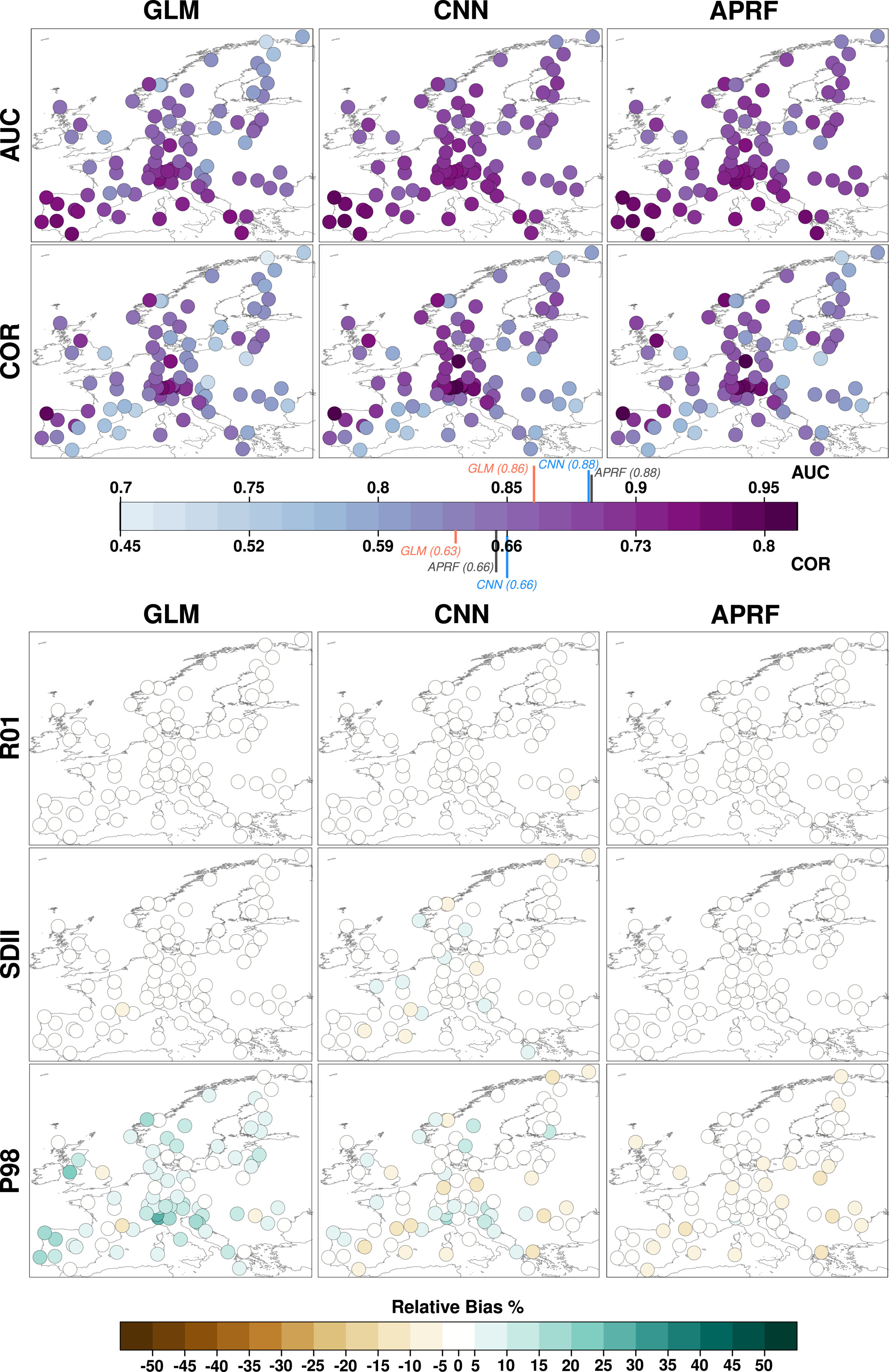
上半部分:AUC & COR(预测能力)
分别衡量降尺度方法在预测降水发生和预测降水量方面的准确性,AUC 和 COR 数值越高,预测能力越强(深紫色代表更好的预测能力,浅蓝色代表较差的预测能力)
作者数值结论如下:
APRF 和 CNN 在 AUC 和 COR 指标上表现类似,均优于 GLM:
AUC 平均值:GLM (0.861) < CNN (0.886) ≈ APRF (0.886)
COR 平均值:GLM (0.63) < CNN (0.662) ≈ APRF (0.657)
GLM 在某些站点表现特别差(如挪威 Karasjok,AUC/COR 仅 0.74/0.46)
CNN 和 APRF 之间的差距不大,说明 CNN 的卷积层并没有提供显著的附加价值,相比之下,APRF 计算成本更低。
预测能力对比(AUC & COR)
下半部分R01, SDII & P98(分布模拟能力):负偏差(肉黄橙色)表示模型低估了降水指标,正偏差(灰色黑色)表示模型高估了降水指标。颜色越深,偏差越大,说明模型误差较大。
作者结论如下:R01(天数预测准不准)三种方法在R01指标上都表现良好,图上几乎没有明显颜色,说明它们都能准确模拟降水发生的频率。SDII(平均降水量预测准不准)CNN的误差较大,部分站点高估降水量,部分站点低估降水量。P98(极端降水)所有方法在P98指标上都存在偏差,但APRF表现最好。
降水分布模拟能力(R01、SDII & P98)
3.2 Downscaling in Non-Perfect Conditions: EC-Earth Historical Scenario
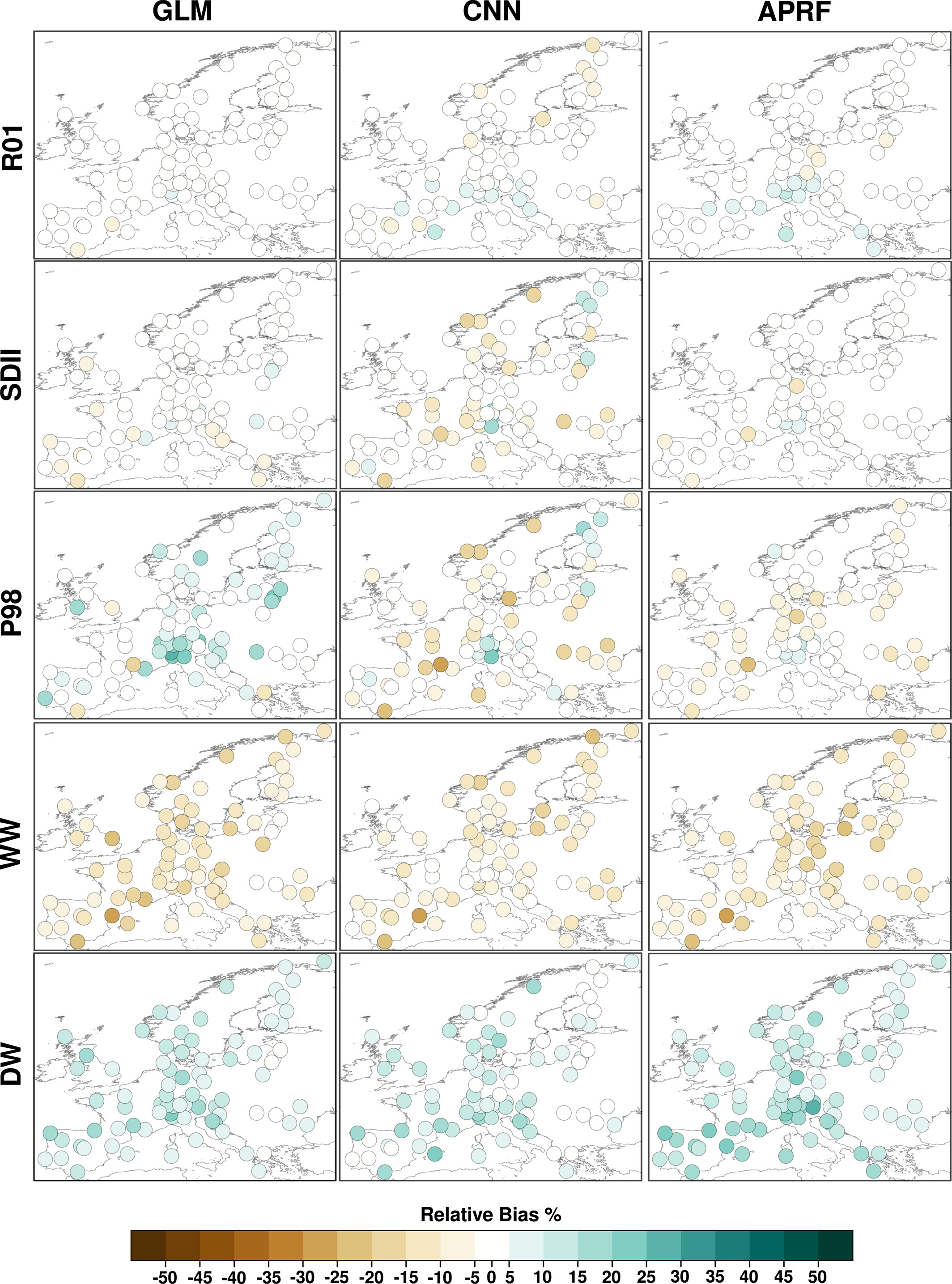
三种 SD 方法在非完美条件下的降尺度偏差(Relative Bias %)
在 非完美条件(使用再分析数据训练,但用于降尺度 EC-Earth GCM 数据)下的相对偏差(Relative Bias),颜色越深,偏差越大
SDII: CNN 误差最大,某些站点偏差高达 ±25%,GLM 和 APRF 误差较小,APRF 在多数站点表现更好。
P98: 确实是 APRF 更好
WW(湿润天后仍然湿润的概率): 所有方法都低估 WW,三种方法都未能正确再现降水持续性。不是前面说这个相关性低不再讨论了吗?
DW(干燥天后仍然干燥的概率):三种方法都倾向于高估干燥天数,这也是 3.4 节 TAPRF 进行改进的原因。
GLMs, CNNs, and APRFs underestimate WW by −11%, −8.2%, and −10.2% and overestimate DW by 9.7%, 8.3%, and 12.9%, respectively. This is the reason motivating the introduction of TAPRFs, a small modification to APRFs which improves this aspect